1. Introduction
Nowadays, Generative AI has become a household name, particularly in the realm of image synthesis—a field that many find captivating and regard as a new creative revolution. However, the ability of models to generate data is far from a recent development. Long before Diffusion Models emerged as the "shining stars" of this domain, several other generative paradigms had already been established, such as Generative Adversarial Networks (GANs), Variational Autoencoders (VAEs), and Normalizing Flow Models (Flow-based models). Each of these approaches employs a distinct methodology to simulate and synthesize realistic novel data.
Among these, if you have prior experience with VAEs, grasping the core concepts of Diffusion Models becomes significantly more intuitive. The rationale behind this is that both frameworks are built upon the ideas of encoding and reconstructing data, utilizing noise as a fundamental component of the learning process. Nevertheless, these are merely foundational similarities—as we delve deeper, it becomes evident that Diffusion Models possess a unique operational philosophy and far greater power. Indeed, these very distinctions have allowed Diffusion Models to break through, serving as the backbone for world-renowned generative systems such as Stable Diffusion, DALL·E, and Midjourney.
So, what exactly makes Diffusion Models so compelling? Fundamentally, they operate on a fascinating principle: the incremental addition of Gaussian noise to real data until the original information is completely transformed into pure noise. Subsequently, the model is trained to master the reverse process—effectively learning to "reclaim the original data" from this chaotic state . One can visualize this as a time-lapse of an image blurring into obscurity, followed by a model learning to sharpen it back to its original state, step by step. Once sufficiently trained, the model can take any random noise sample and iteratively "restore" it into a complete, sharp, and natural-looking image.
While this may sound straightforward, a common question arises: "How can a simple text prompt like 'a cat riding a bicycle in space' lead to the generation of a cinematic, sci-fi masterpiece?" This is where the magic of guidance mechanisms occurs. During the denoising training phase, the model is provided with additional information from the prompt in the form of embedding vectors. In other words, the model does not merely learn to reconstruct data; it learns to steer that reconstruction based on natural language instructions. This enables Diffusion Models to "understand" prompt content and translate it into a corresponding visual representation.
In the following sections, I will lead you on a deep dive into how Diffusion Models learn, how they handle noise, and why they are capable of producing such stunning, emotionally resonant, and detailed imagery. For now, let us begin with the primary question: What exactly are Diffusion Models, and why has the AI world focused its attention so intensely on them?
Below is a summary of the upcoming sections:
- Generative Mechanism: We will explore the fundamental principles of how Diffusion Models operate, including the forward and reverse processes that govern their functionality.
- Theoretical Foundations: This section will delve into the mathematical and theoretical underpinnings of Diffusion Models, providing insights into why they work so effectively.
- Optimization Inference: We will discuss various techniques to optimize the inference process, making it more efficient without sacrificing quality.
- Guidance Mechanism: This part will explain how guidance mechanisms enable models to generate content based on specific prompts, enhancing their versatility and control.
- Conclusion: Finally, we will summarize the key takeaways and discuss the future prospects of Diffusion Models in generative AI.
2. Generative Mechanism
2.1 Theoretical Probability and Statistical Mechanics
Random Variable
Any real-valued mapping that takes a sample space $\Omega$ as its domain, specifically $X:\Omega\longrightarrow\mathbb{R}$, is defined as a random quantity, or more concisely, a random variable. In this context, $X$ maps each outcome $\omega\in\Omega$ to a corresponding real number $X(\omega)$.
Cumulative Distribution Function (CDF)
Let $X$ be a random variable. The distribution function (or Cumulative Distribution Function) of $X$ is defined by: $$F(u) = P(X \le u)$$
Probability Density Function (PDF)
Let $X$ be a random variable; there exists an integrable function $f(u)$ such that for any $a, b \in \mathbb{R}$: $$P(a < X < b) = \int_{a}^{b} f(u) du$$ Furthermore, if $F(u)$ is differentiable, we have: $$f(u) = F'(u)$$
Expectation (Expected Value)
Let $X$ be a random variable with a probability density function $f$. The expectation (or expected value) of $X$ is then defined by: $$\mu = E(X) = \int_{-\infty}^{+\infty} x f(x) dx$$
Variance
Let $X$ be a random variable with an expected value $m = E(X)$. The variance of $X$ is defined as: $$\sigma^2 = V(X) = E[(X - m)^2]$$ In the multivariate case, we represent this as the Covariance Matrix, denoted by the symbol $\Sigma$.
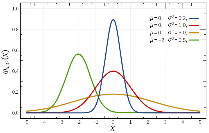
Normal Distribution (Gaussian Distribution)
A random variable $X$ is said to have a normal distribution $\mathcal{N}(\mu, \sigma^2)$ if it has the following probability density function : $$f(x) = \frac{1}{\sigma\sqrt{2\pi}}e^{-\frac{(x-\mu)^2}{2\sigma^2}}$$ If $\mu=0$ and $\sigma=1$, then $\mathcal{N}(0,1)$ is referred to as the standard normal distribution, and its density function is denoted by $\phi$.
Law of Large Numbers (LLN)
The sample mean converges to the population expectation as the sample size becomes sufficiently large . Mathematically, this is expressed as: $$\lim_{n\to\infty} \overline{X}_n = \mu$$
Central Limit Theorem (CLT)
The sample mean $\overline{X}_n$, derived from $n$ random observations of ANY arbitrary distribution, can always be approximated by a normal distribution $\mathcal{N}(\mu, \frac{\sigma^2}{n})$ : $$\lim_{n\to\infty} P\left(\frac{\overline{X}_n - \mu}{\sigma/\sqrt{n}} \le u\right) = \Phi(u)$$
Parameter Estimation for Arbitrary Distributions
Leveraging the Law of Large Numbers and the Central Limit Theorem, we can estimate the parameters of any distribution by assuming it follows a normal distribution, provided that the sample size is SUFFICIENTLY LARGE.
2.2 Deep Learning from a Statistical Perspective
The Universal Approximation Theorem
The Universal Approximation Theorem states that a feedforward neural network with a single hidden layer and a finite number of neurons can approximate any continuous function on a compact subset of the real numbers $\mathbb{R}^n$, given an appropriate activation function. (GeeksforGeeks)
Encoding Real-World Data
We maintain the observation that if real-world data can be encoded into a computable space, then the process of "learning" in a deep learning model is essentially the estimation of a function capable of generalizing across that entire space.
Generative AI
Generative AI represents a unique paradigm: rather than estimating a standard, deterministic function, we focus on estimating the underlying probability distribution of the data. Consequently, generating novel data from this learned distribution is fundamentally equivalent to the process of stochastic sampling.
To understand the rationale behind distribution estimation, consider the visualization of cat images (as seen on Figure 2). Suppose we possess a generative model designed to produce images of cats. If the model were based on standard function estimation, it would lack randomness across different iterations; in other words, every generated image would be identical. This would result in a loss of the "creativity" that generative systems are intended to achieve.
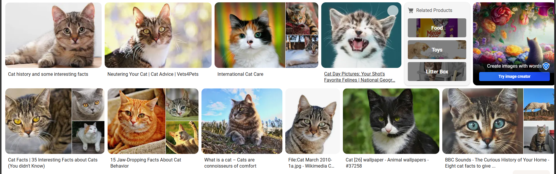
Conversely, by estimating a probability distribution, each sampling instance yields distinct variations. This ensures that while the output is consistently recognizable as a cat, every generated result remains unique and diverse.
2.3 Generative Models
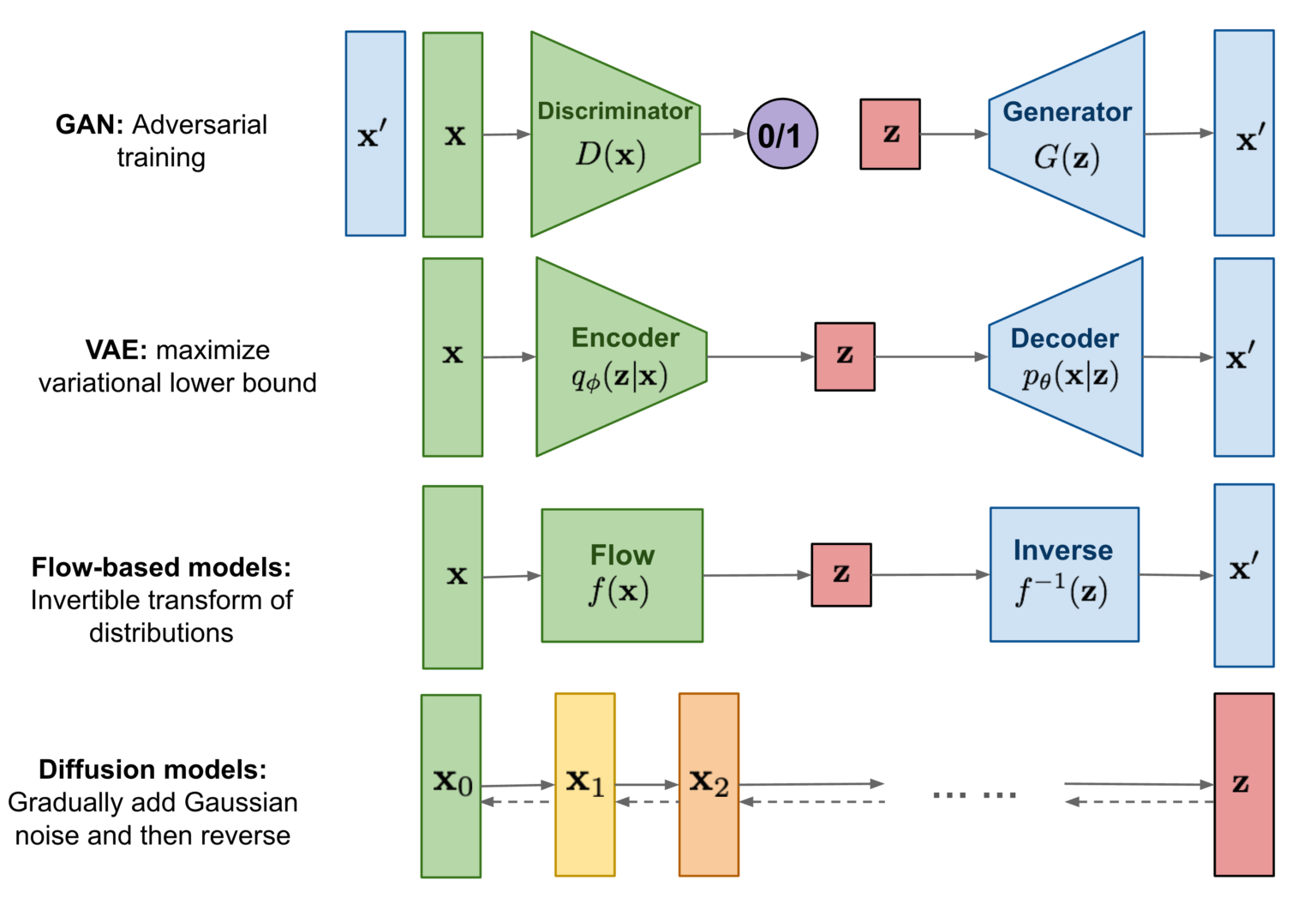
Generative Adversarial Networks (GANs)
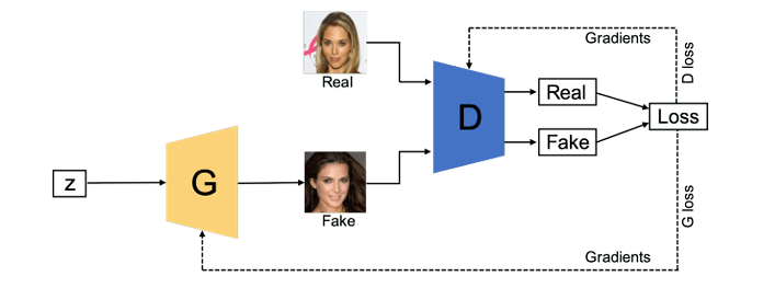
GANs (Ian et al., 2014) consist of two neural networks, a generator and a discriminator, that are trained simultaneously through an adversarial process. The generator creates fake data samples, while the discriminator evaluates them against real data, providing feedback to improve the generator's output.
Variational Autoencoders (VAEs)
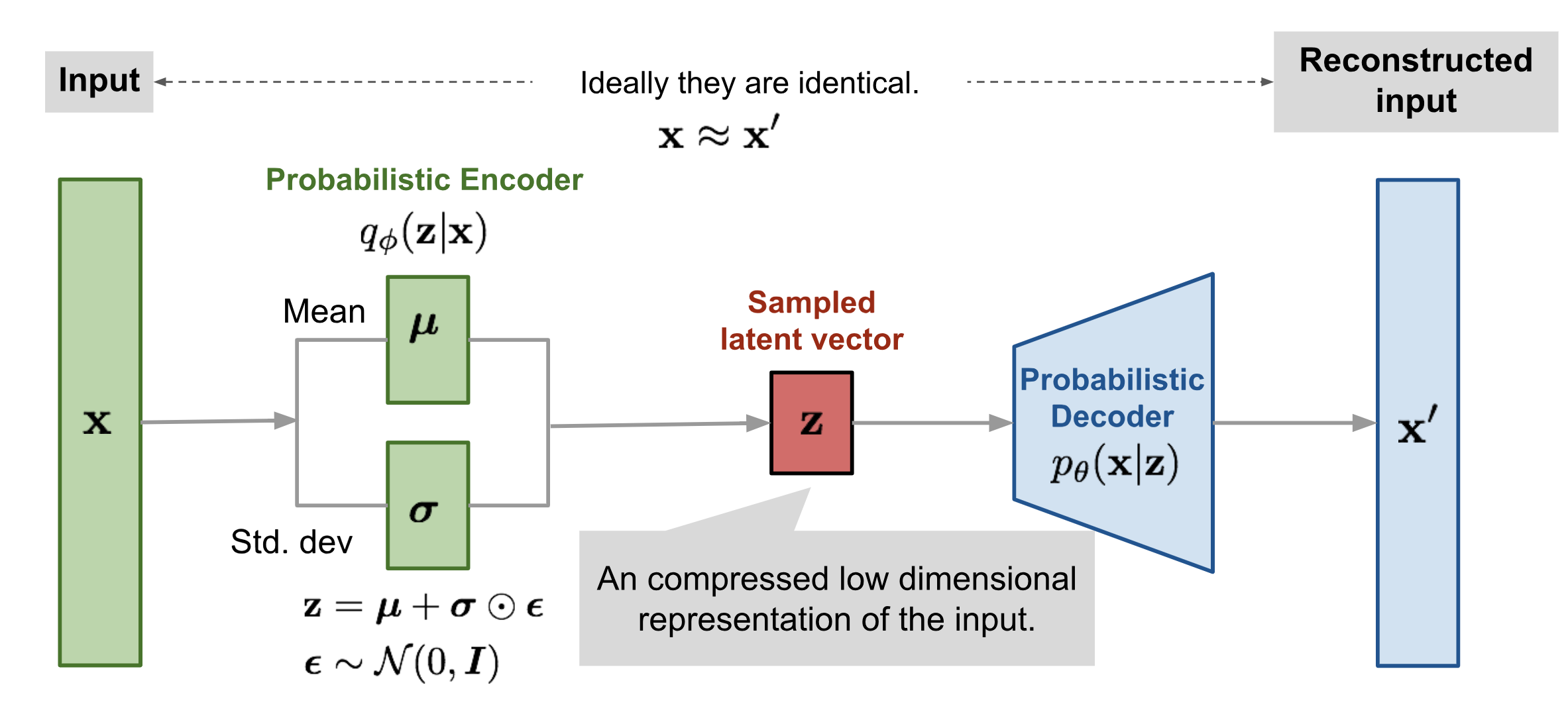
VAEs (Kingma and Welling, 2013) are a type of generative model that learns to encode input data into a latent space and then decode it back to the original space. They optimize a variational lower bound on the data likelihood, allowing for efficient sampling and generation of new data.
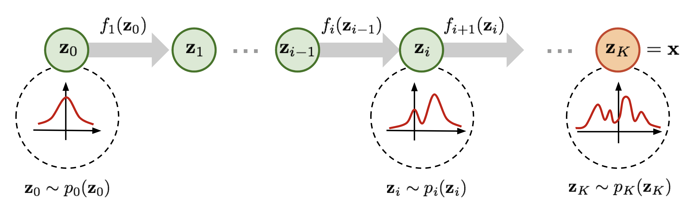
Normalizing Flow Models
Normalizing flow models (Dinh et al., 2015) transform a simple probability distribution (like a Gaussian) into a more complex one by applying a series of invertible transformations. This allows for exact likelihood estimation and efficient sampling.
Diffusion Models
Diffusion Models (Chieh-Hsin et al., 2025) operate by gradually adding noise to data until it becomes pure noise, and then learning to reverse this process to generate new data. They have shown remarkable performance in generating high-quality images and other types of data.
2.4 Diffusion Models
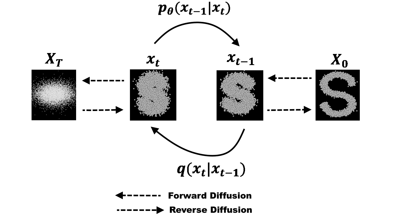
Forward Process
The Forward Diffusion Process involves the systematic destruction of data across multiple time steps by incrementally injecting Gaussian noise at each interval. This process is mathematically formulated as follows: $$q(x_t|x_0) = \mathcal{N}(x_t; \sqrt{\alpha_t}x_0, (1-\alpha_t)\mathbf{I})$$ Using the reparameterization trick, we can express the noisy state $x_t$ directly as: $$x_t = \sqrt{\alpha_t}x_0 + \sqrt{1-\alpha_t}\epsilon$$ where $\epsilon \sim \mathcal{N}(0, \mathbf{I})$ represents the Gaussian noise added at each step and $\alpha_t$ follows a predefined schedule that governs the gradual degradation of the data over time.
Reverse Process
Conversely, the Reverse Diffusion Process (or Diffusion Inversion) refers to the reconstruction phase where the model learns to restore structured data from noise back to its original state. This step-by-step recovery is modeled as: $$p_\theta(x_{t-1}|x_t) = \mathcal{N}(x_{t-1}; \mu_\theta(x_t, t), \Sigma_\theta(x_t, t))$$
It can be observed that the forward process of adding noise can be viewed as a data labeling procedure, where the added noise itself serves as the label. The reverse process then involves training a model to predict this noise; however, I will not delve into the specific mathematical nuances of why noise prediction is effective in this post.
At first glance, because each state depends recursively on the one preceding it, it would seem that knowing the original data point, $x_0$, is a prerequisite for reconstruction. Yet, during the inference phase, knowing $x_0$ is virtually impossible and computationally infeasible. Fortunately, it has been proven that we only need two specific quantities—the state at time $t$ ($x_t$) and the predicted noise ($\epsilon_t$)—to execute the reverse process successfully without requiring the original $x_0$ .
Beyond noise prediction, researchers have also demonstrated that data can be reconstructed using velocity fields. This approach is closely related to a cutting-edge technology known as Flow Matching, which provides a more direct path for data generation. I look forward to exploring the intricacies of Flow Matching in a separate blog post.
The Training Objective
To master the reconstruction, the model minimizes a simplified loss function, which measures the discrepancy between the added noise and the noise predicted by the neural network: $$L_{simple} = E_{x_0, \epsilon, t} \left[ \left\| \epsilon - \epsilon_\theta(\sqrt{\alpha_t}x_0 + \sqrt{1-\alpha_t}\epsilon, t) \right\|^2 \right]$$
2.5 Diffusion Model Architecture
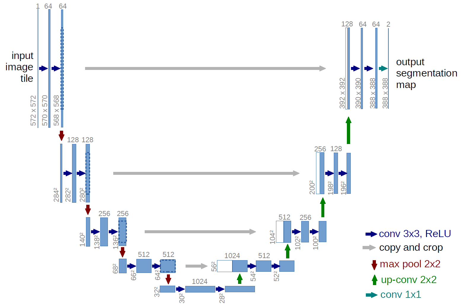
U-Net Architecture
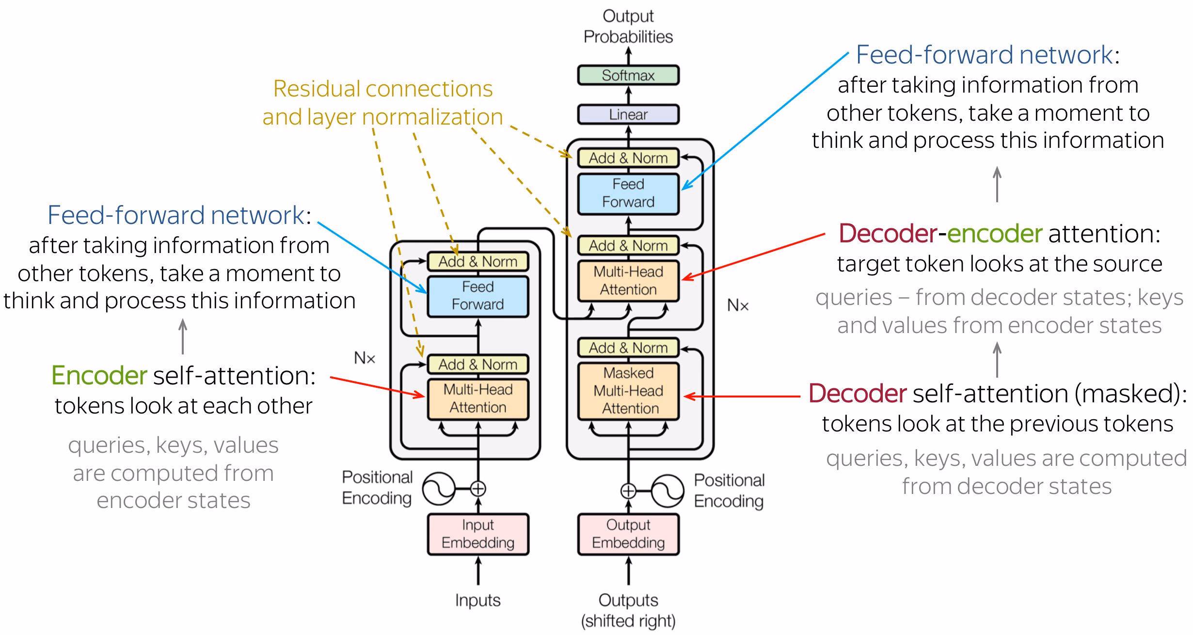
Transformer Architecture
3. Theoretical Foundations
3.1 A Triple Perspective on the Foundations of Diffusion Models
A Statistical Physics Perspective: Nonequilibrium Thermodynamics
A relatively novel idea involves explaining the operational principles of Diffusion Models as a Nonequilibrium Dynamical System. This concept was first introduced in 2015 in the seminal paper "Deep Unsupervised Learning using Nonequilibrium Thermodynamics" by Sohl-Dickstein et al. (2015). In this work, the authors define the forward process as a Markov chain $q(x_t|x_{t−1})$; those familiar with Reinforcement Learning will find the concept of a Markov chain quite recognizable. At each time step $t$, Gaussian noise is incrementally added to this distribution—the Markov chain. Remarkably, it has been mathematically proven that as time $T$ increases, the distribution $q$ asymptotically approaches a standard normal distribution $N(0,I)$. Converting data into a Normal or "white" noise distribution is an exceptionally promising approach, as the Normal distribution is highly favored for its efficiency, and the vast majority of modern machine learning and deep learning algorithms operate under the assumption that data follows a Gaussian distribution.
In other words, as $t \to T$, the diffusion process completely obliterates the structure of the original data, rendering every sample $x_T$ as pure Gaussian noise. Consequently, the authors interpret this from a statistical physics perspective as a nonequilibrium thermodynamic process. In this framework, the system's entropy increases over time until it reaches a state of equilibrium—specifically, the isotropic Gaussian distribution $N(0,I)$.
Following the definition of the forward diffusion process, which dismantles the data structure, Sohl-Dickstein demonstrated that a reverse process can be constructed to reconstruct data from noise. This is known as the reverse diffusion process, which serves as the generative mechanism (generative process) of the model. In statistical physics, if the complete dynamics of the forward diffusion process are known, it is theoretically possible to simulate a corresponding time-reversal process—meaning a system gradually transitions from a high-entropy Gaussian noise state back to a structured, low-entropy state. However, because the forward diffusion process is a nonequilibrium process, a direct and exact reversal is not possible. Instead, the model learns an approximation of these reverse dynamics through parameterization using neural networks. After completing $T$ denoising steps, we obtain a sample $x_0$ that follows the same distribution as the original training data. This process can be conceptualized as traveling back in time relative to the forward diffusion process—effectively transforming Gaussian noise into structured, meaningful data.
A Variational Inference Perspective: From VAEs to Hierarchical VAEs
Next, we explore another perspective on Diffusion Models through the evolution of architectures commonly referred to as U-Nets or Encoder-Decoder structures. Consequently, if you investigate Variational Autoencoders (VAEs) beforehand, you will notice a significant connection between them and Diffusion Models that warrants clarification. While the Encoder-Decoder mechanism shares foundational similarities, the primary distinction lies in how noise is introduced. Following VAEs, researchers developed Hierarchical VAEs (HVAEs), a model that is closely related to Diffusion Models. In fact, Diffusion Models can be characterized as a specialized case of Hierarchical Variational Autoencoders, typically assuming $\epsilon \sim \mathcal{N}(0, \mathbf{I})$.
In VAEs, the encoder learns to map the input $x$ into a latent representation $z \sim \mathcal{N}(\mu, \sigma^2)$, effectively estimating the distribution $q_\theta(z|x)$. The decoder subsequently learns to reconstruct $x$ from $z$, estimating the distribution $p_\phi(x|z)$. Image generation in VAEs involves sampling from the learned distribution, expressed as $z = \mu_\theta + \sigma_\theta \times \epsilon$. This mechanism requires training two separate neural networks: an encoder for downsampling and a decoder for upsampling, with noise only introduced at the latent stage to ensure stochasticity .
In HVAEs, the encoder learns to map $x$ to a series of latent variables $z_i \sim \mathcal{N}(\mu_i, \sigma_i^2)$, requiring the estimation of $\mu_i$ and $\sigma_i^2$ at each stage $i$. The decoder then learns to decode each stage $i$ in a manner corresponding to the encoder. Similar to VAEs, generation is achieved by sampling from the encoder's distributions, such that $z_i = \mu_i + \sigma_i \times \epsilon$. While HVAEs inject noise at every stage $i$ of the encoder, maintaining two full networks for both encoding and decoding remains computationally expensive.
Finally, Diffusion Models simplify this paradigm by bypassing the explicit encoder entirely and adding noise directly to the raw data. The decoder then learns to reconstruct the data from this noisy input. This approach represents a strategic trade-off: accepting a marginal decrease in accuracy for a significant increase in the efficiency of the forward process. As previously mentioned, further refinements involve predicting the added noise rather than the sample at step $t$ to enhance model performance.
A Score-Based Perspective: From Score Matching to Stochastic Differential Equations
Beyond the perspectives of Thermodynamics or VAEs, Diffusion Models can be approached through a fascinating mathematical lens: Differential Calculus. This framework focuses on learning the geometric structure of data through the concept of the Score Function.
In statistics, the Score function of a distribution $p(x)$ is defined as the gradient of the log-density with respect to the data $x$: $$s(x) = \nabla_x \log p_{data}(x)$$ eometrically, $s(x)$ represents a vector field indicating the direction of the steepest increase in data density. If the data space is envisioned as a map, the Score function acts as a "guide," leading us from regions of pure Gaussian noise back to the manifold where real data resides.
However, a significant challenge arises: the Manifold Hypothesis. This hypothesis suggests that real-world data typically resides on low-dimensional manifolds within a high-dimensional space, meaning the score function $\nabla_x \log p_{data}(x)$ is not globally defined. To address this, Song & Ermon (2019) proposed the Noise Conditional Score Network (NCSN). Instead of learning the score function of the original data, they perturb the data with various noise levels $\sigma$ and train a single neural network to approximate the score function across all noise levels: $$s_\theta(x, \sigma) \approx \nabla_x \log q_\sigma(x)$$ This strategy allows the model to "perceive" the correct direction even when positioned far from the actual data manifold.
Once the "guide" $s_\theta$ is established, sample generation is performed via Annealed Langevin Dynamics (ALD). This process begins at high noise levels and gradually decreases (akin to simulated annealing in physics), enabling the sample to transition intelligently from a chaotic state back to structured data.
A pivotal breakthrough occurs when we recognize that both the Forward and Reverse processes are essentially equivalent to solving Differential Equations.
- SDE (Stochastic Differential Equation): Describes the diffusion process as a random system, similar to Brownian motion within a force field.
- ODE (Ordinary Differential Equation): The perspective offered by DDIM (Jiaming Song et al., 2020) allows us to transform the stochastic process into a deterministic trajectory, thereby accelerating sampling without compromising image fidelity.
The unification of score-based models and probabilistic diffusion models via the Reverse-time SDE framework has established a robust foundation for contemporary technologies, most notably Flow Matching—a technique promising the most optimal "straight paths" connecting noise to real data.
4. Optimization Inference
4.1 Latent Space Optimization
Latent Diffusion Models
Traditional diffusion operates directly in the high-dimensional pixel space, making the generation of high-resolution images computationally prohibitive.
- Latent Diffusion Models (LDMs) (Robin et al., 2022) address this issue by performing the diffusion process in a lower-dimensional latent space. This is achieved by first encoding the input data into a compact latent representation using an autoencoder, and then applying the diffusion process within this latent space. The decoder subsequently reconstructs the high-resolution image from the denoised latent representation, significantly reducing computational costs while maintaining high-quality outputs.
4.2 Deterministic Sampling
Denoising Diffusion Implicit Models (DDIM)
Standard DDPM sampling is inherently stochastic (random) and requires hundreds of Markovian steps (often $T=1000$) to produce a single image, leading to extremely slow inference speeds.
- Denoising Diffusion Implicit Models (DDIM) (Jiaming Song et al., 2020) introduce a non-Markovian, deterministic sampling process that significantly accelerates inference. By reparameterizing the reverse diffusion process, DDIM allows for fewer sampling steps (as low as $T=50$) without compromising image quality, making it a practical choice for real-world applications.
5. Guidance Mechanism
5.1 Guidance Problem
Suppose we aim to generate an image based on a specific prompt; in this context, the prompt represents our desired intent. Formally and generally, this involves learning a conditional distribution expressed as (Prafulla Dhariwal and Alex Nichol, 2021): $$\nabla_x \log p_{data}(x|y) = \nabla_x \log p_{data}(x) + \nabla_x \log p_{data}(y|x)$$ The component $\nabla_x \log p_{data}(y|x)$ is referred to as the classifier. Consequently, the score function acts not only as a "guide" for the most efficient path but also ensures that the trajectory leads toward the most accurate outcome.
Classifier Guidance
This method utilizes the gradient of a pre-trained classifier to "steer" the diffusion process toward a target label. It is analogous to performing an adversarial attack on the classifier to compel the model to synthesize images that strictly belong to the correct class (Prafulla Dhariwal and Alex Nichol, 2021): $$\hat{\epsilon}(x_t) = \epsilon_\theta(x_t) - \sqrt{1-\bar{\alpha}_t} \cdot s \cdot \nabla_{x_t} \log p_\phi(y|x)$$ In this equation, $s$ denotes the gradient scale factor.
Classifier-Free Guidance
Instead of training an auxiliary classifier, this approach incorporates the conditioning information directly into the training phase alongside noise prediction. It employs a linear combination between the conditional prediction $\epsilon_\theta(z_\lambda, c)$ and the unconditional prediction $\epsilon_\theta(z_\lambda)$. This mechanism strives to push the sample toward the conditional distribution while simultaneously pulling it away from the unconditional one (Jonathan Ho and Tim Salimans, 2021): $$\hat{\epsilon}_\theta(z_\lambda, c) = (1+w)\epsilon_\theta(z_\lambda, c) - w\epsilon_\theta(z_\lambda)$$ Here, $w$ represents the guidance weight.
6. Conclusion
In this article, we have explored the intricate workings of Diffusion Models, a powerful class of generative models that have revolutionized the field of AI-driven content creation. We delved into their generative mechanism, theoretical foundations, optimization techniques, and guidance mechanisms that enable them to produce stunning and contextually relevant outputs. As we look to the future, it is clear that Diffusion Models will continue to play a pivotal role in advancing generative AI, opening new avenues for creativity and innovation across various domains.