Advanced Diffusion Models

1. Introduction

The journey began by framing image generation as a latent variable model problem. In this initial stage, Denoising Diffusion Probabilistic Models (DDPM) leveraged the Evidence Lower Bound (ELBO) to optimize the reversal of a Markovian noise process. The core objective was centered on '$\epsilon$-prediction,'' where a neural network learned to estimate and subtract noise step-by-step to recover the data distribution.

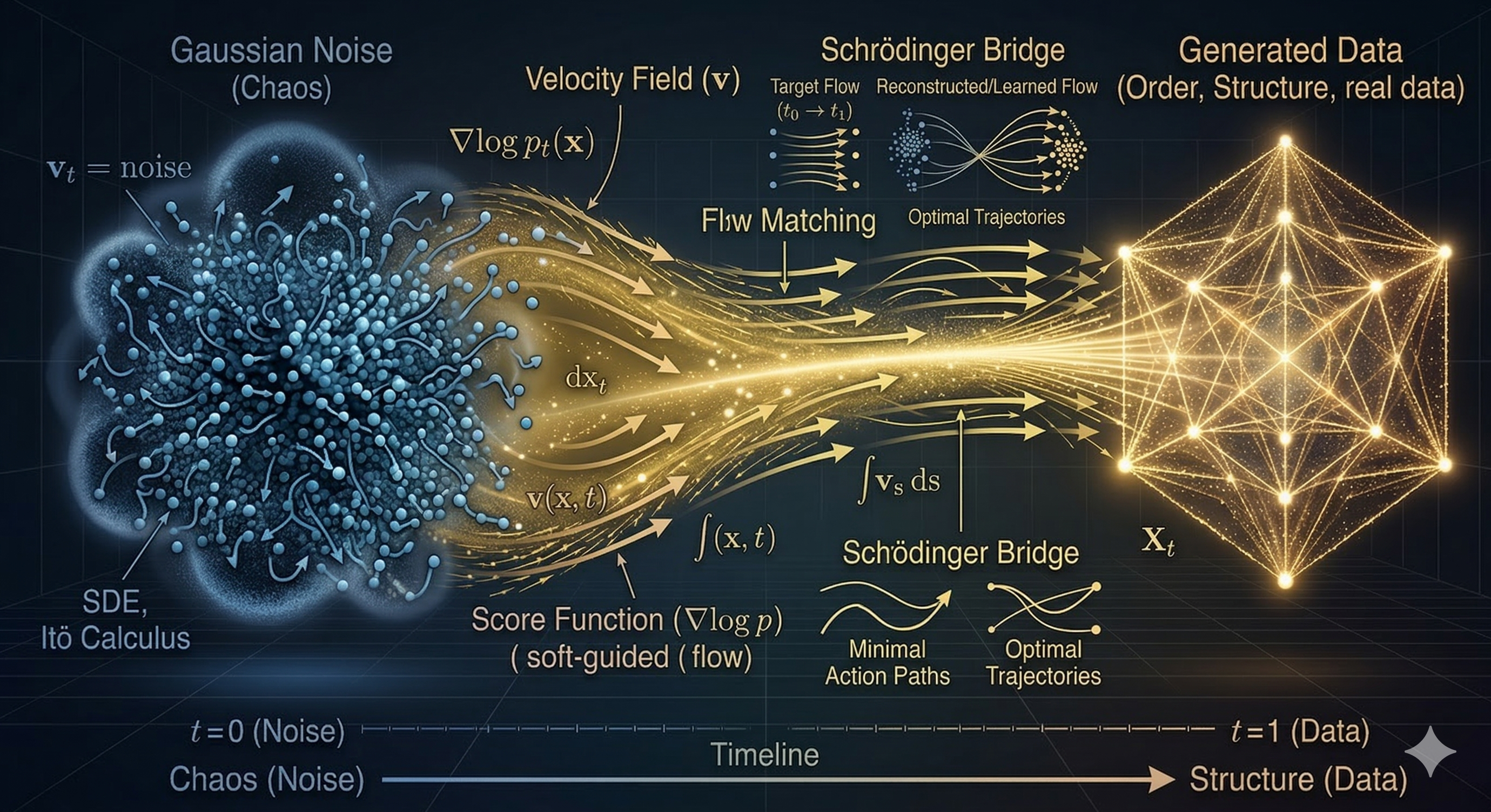
As the field matured, researchers shifted from discrete steps to continuous-time modeling. By employing Stochastic Differential Equations (SDEs) and Itô calculus, the diffusion process was reimagined as a continuous evolution of data particles within a random force field. This transition allowed for a more rigorous mathematical treatment of how data density transforms over time.

A major theoretical leap occurred with the introduction of the Fokker-Planck equation. Instead of tracking individual particles, this perspective focused on the evolution of the entire probability density. It provided the mathematical proof that for every stochastic process (SDE), there exists a corresponding deterministic flow—the Probability Flow ODE—that results in the exact same marginal distributions.

With the foundation of Fokker-Planck, the paradigm shifted from 'denoising' to 'navigation.' The goal became finding the optimal Velocity Field ($v$) to guide data points along a specific trajectory. This marked the birth of velocity-based learning, where the network predicts the direction and speed of data movement rather than just the noise component.

Flow Matching emerged to clean up and unify the diverse landscape of generative objectives (noise, data, score, and velocity). This era introduced Rectified Flows, which 'straighten' the curved paths of traditional diffusion. By enforcing straight-line trajectories, Flow Matching minimized transport costs and enabled high-quality sampling in significantly fewer steps.

To further optimize these paths, the Schrödinger Bridge problem was revisited. This addressed the challenge of transitioning between two distributions (A to B) with minimum energy expenditure and optimal entropy within a finite timeframe. This connection to Optimal Transport theory allowed for direct image-to-image translations and more efficient couplings between arbitrary distributions without strictly relying on a Gaussian prior.

We are currently entering the era of Generator Matching (GM), the 'Grand Unified Theory' of generative modeling. GM acts as a meta-framework that encompasses Diffusion, Flow, and even discrete Jump processes. By utilizing the infinitesimal generator ($\mathcal{L}$), it defines all forms of data transformation within a single mathematical operator. This facilitates the creation of truly unified multimodal systems where any data type can be modeled as a flow on a geometric manifold.

Below is a summary of the upcoming sections:

• Section 2 - From Vector Fields to Score Functions: Bridging the gap between deterministic vector calculus and stochastic score matching, illustrating how score functions dictate the gradient of log-density in diffusion processes.
• Section 3 - Divergence and the Continuity Equation: Formulating the conservation of probability mass. We will derive the Fokker-Planck equation and demonstrate how the Probability Flow ODE perfectly mirrors the marginal distributions of its SDE counterpart.
• Section 4 - Advanced Perspectives (Flow Matching): Unifying various prediction targets (noise, data, score, and velocity parameterizations) and introducing the Flow Matching framework as a method to construct straight, tractable probability paths.
• Section 5 - Optimal Transport and Schrödinger Bridges: Exploring the geometric and thermodynamic limits of generative models. We will examine how Optimal Transport yields straightest-path generation, while Schrödinger Bridges solve the entropy-regularized boundary problem for optimal stochastic routing.
• Section 6 - Sampling and Conditional Control: Investigating how conditional variables mathematically steer the probability flow. This section breaks down the mechanics of Classifier-Free Guidance (CFG) as a vector extrapolation technique in the latent space.
• Section 7 - Sophisticated Solvers (DPM-Solvers): Transitioning from theoretical continuous flows to practical numerical implementation. We analyze how Exponential Integrators isolate the linear drift from the non-linear neural network, drastically reducing the required number of function evaluations (NFE).
• Section 8 - Consistency Models: The ultimate leap towards real-time generation. We detail how enforcing a global self-consistency mapping allows neural networks to bypass iterative ODE solving, teleporting any point on a trajectory directly to the pristine data in a single step.

2. From Vector Field to Score Functions

2.1 Multivariable Calculus

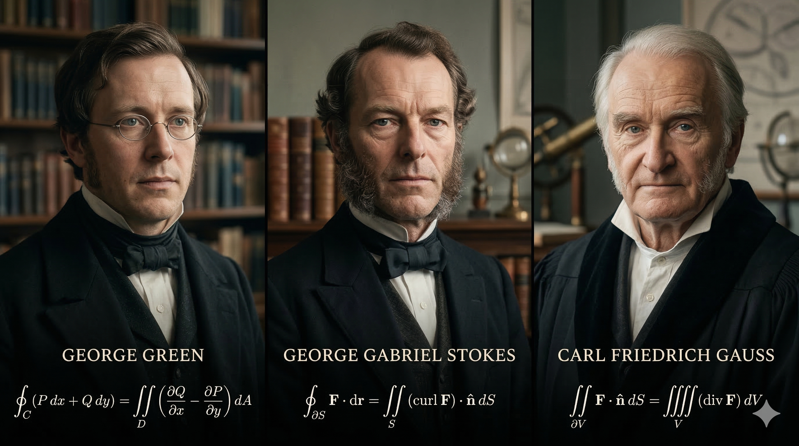
Multivariable calculus serves as a crucial mathematical foundation for this blog. I sincerely advise readers to revisit this subject—especially vector calculus—if they do not yet have a profound understanding of it, before proceeding to the subsequent sections. I would like to recommend a wonderful book, and my personal favorite on the topic: Multivariable Calculus by Don Shimamoto (Don Shimamoto, 2019). Readers should clearly master the three fundamental theorems of vector calculus: Green's Theorem for line integrals, Stokes' Theorem (which bridges line and surface integrals), and the famous Gauss's Theorem (Divergence Theorem). Furthermore, a solid grasp of differential equations and their solutions will ensure you do not feel overwhelmed by the complex formulas in the later chapters.

2.2 Vector Fields

Definition of Vector Fields

Conservative Fields

Line Integrals

2.3 Score Functions

Definition of Score Functions

“Suppose our dataset consists of i.i.d. samples $\{x_i \in \mathbb{R}^d\}_{i=1}^N$ from an unknown data distribution $p_{data}(x)$. We define the score of a probability density $p(x)$ to be $\nabla_x \log p(x)$. The score network $s_\theta: \mathbb{R}^D \to \mathbb{R}^D$ is a neural network parameterized by $\theta$, which will be trained to approximate the score of $p_{data}(x)$. The goal of generative modeling is to use the dataset to learn a model for generating new samples from $p_{data}(x)$. The framework of score-based generative modeling has two ingredients: score matching and Langevin dynamics.” (Yang Song & Stefano Ermon, 2019)

The definition of the Score Function as $\nabla_x \log p(x)$ is not an arbitrary choice; it is a mathematically strategic definition that solves the most fundamental problem in generative modeling: the intractability of the partition function. Here is why Yang Song and Stefano Ermon (building on the work of Aapo Hyvärinen) use this specific formulation.

Bypassing the Partition Function ($Z$). In traditional generative modeling, a probability density function is often expressed as: $$p(x) = \frac{\tilde{p}(x)}{Z}$$ Where $\tilde{p}(x)$ is the unnormalized density (the part the model can calculate) and $Z = \int \tilde{p}(x) dx$ is the partition function (the normalization constant).

In high-dimensional spaces, calculating $Z$ is nearly impossible because it requires integrating over all possible values of $x$. By taking the gradient of the log-density, we get: $$\nabla_x \log p(x) = \nabla_x \log \left( \frac{\tilde{p}(x)}{Z} \right) = \nabla_x \log \tilde{p}(x) - \nabla_x \log Z$$ Since $Z$ is a constant with respect to $x$, its gradient is zero ($\nabla_x \log Z = 0$). Therefore: $$\nabla_x \log p(x) = \nabla_x \log \tilde{p}(x)$$ So, the Score Function allows us to learn the structure of the data distribution without ever needing to calculate the impossible normalization constant $Z$.

The Score as a Vector Field of Direction. Mathematically, the gradient $\nabla_x$ points in the direction of the steepest increase of a function. By defining the score as $\nabla_x \log p(x)$, we create a vector field that always points toward regions of higher data density. In regions where there is no data, the score points toward the data manifold. At the 'peaks' (modes) of the distribution, the score becomes zero. This makes the score function a perfect 'guide' for moving noise towards data.

Connection to Langevin Dynamics. The second 'ingredient' mentioned in your text is Langevin Dynamics. This is a stochastic process used for sampling. The update rule is: $$x_{t+1} = x_t + \epsilon \nabla_x \log p(x) + \sqrt{2\epsilon} z_t$$ In this physical analogy, the Score Function acts as a force field. It 'pushes' the sample $x$ toward the high-probability regions of $p_{data}(x)$, while the $z_t$ term adds a bit of random 'jitter' to ensure the sampler explores the whole distribution rather than getting stuck in one spot. Without the gradient of the log-density, we wouldn't have a mathematical "force" to drive the sampling process.

Fisher Information and Score Matching. Historically, in statistics, $\nabla_\theta \log p(x|\theta)$ is known as the Fisher Score. Song & Ermon adapted this into a spatial score ($\nabla_x$). The reason we can train a neural network $s_\theta(x)$ to approximate this without knowing $p_{data}(x)$ is through Score Matching. Hyvärinen proved that: $$\mathbb{E}_{p_{data}(x)} [\|\nabla_x \log p_{data}(x) - s_\theta(x)\|^2]$$ Can be rewritten (using integration by parts) into a form that only requires the samples $x_i$ and the derivatives of the neural network, making the 'unknown' $p_{data}$ disappear from the loss function.

Change in Probability (Log-Likelihood)

According to the Fundamental Theorem of Line Integrals, if a vector field $\mathbf{F}$ is conservative (i.e., $\mathbf{F} = \nabla f$), then the line integral along a curve $\alpha$ from point $a$ to point $b$ depends only on the values of the potential function $f$ at the endpoints: $$\int_{\alpha} \nabla f \cdot d\mathbf{s} = f(\alpha(b)) - f(\alpha(a))$$ Applying this theorem to the Score Function: $$\int_{\alpha} \nabla \log p(\mathbf{x}) \cdot d\mathbf{s} = \log p(\mathbf{x}_{final}) - \log p(\mathbf{x}_{initial}) = \log \frac{p(\mathbf{x}_{final})}{p(\mathbf{x}_{initial})}$$

The line integral of the Score Function along a trajectory $\alpha$ represents the total cumulative change in the log-probability of the data as it moves along that path. A positive integral value indicates that the trajectory is moving toward 'more realistic' data regions—areas characterized by higher probability density.

3. Divergence and Continuity Equation

3.1 Gauss's Theorem and Divergence

Definition of Divergence

In the specific case of 3D space ($n=3$), where the vector field is given by $\mathbf{F} = \langle M, N, P \rangle$, the formula simplifies to: $$\text{div } \mathbf{F} = \frac{\partial M}{\partial x} + \frac{\partial N}{\partial y} + \frac{\partial P}{\partial z}$$

Shimamoto describes Divergence as a measure of the 'flux density' or the rate at which a 'fluid' (or probability density) is expanding or contracting at a specific point:

• Source: If $\text{div } \mathbf{F} > 0$ at a point, the field is 'spreading out.' This indicates a source where matter, energy, or probability is being generated or flowing outward.
• Sink: If $\text{div } \mathbf{F} < 0$ at a point, the field is 'compressing.' This indicates a sink where the flow is accumulating or vanishing.
• Incompressible: If $\text{div } \mathbf{F} = 0$, the flow is steady, with no net gain or loss at that point.

Gauss's Theorem

In the context of Diffusion Models, Gauss's Theorem provides a mathematical framework for understanding how local changes in probability density (as measured by divergence) relate to the overall flow of probability mass across space. It helps us analyze how probability 'flows' from low-density regions (sources) to high-density regions (sinks) during the generative process.

3.2 Continuity Equation and Fokker-Planck Equation

Continuity Equation

The Continuity Equation is a fundamental principle in physics that describes the conservation of some quantity (like mass, energy, or probability) as it flows through space and time. In the context of probability density $p(\mathbf{x}, t)$ evolving under a velocity field $\mathbf{v}(\mathbf{x}, t)$, the Continuity Equation can be expressed as: $$\frac{\partial p}{\partial t} + \nabla \cdot (p \mathbf{v}) = 0$$

This equation states that the rate of change of probability density at any point in space and time is balanced by the net flow of probability into or out of that point. It ensures that probability is conserved during the generative process modeled by diffusion.

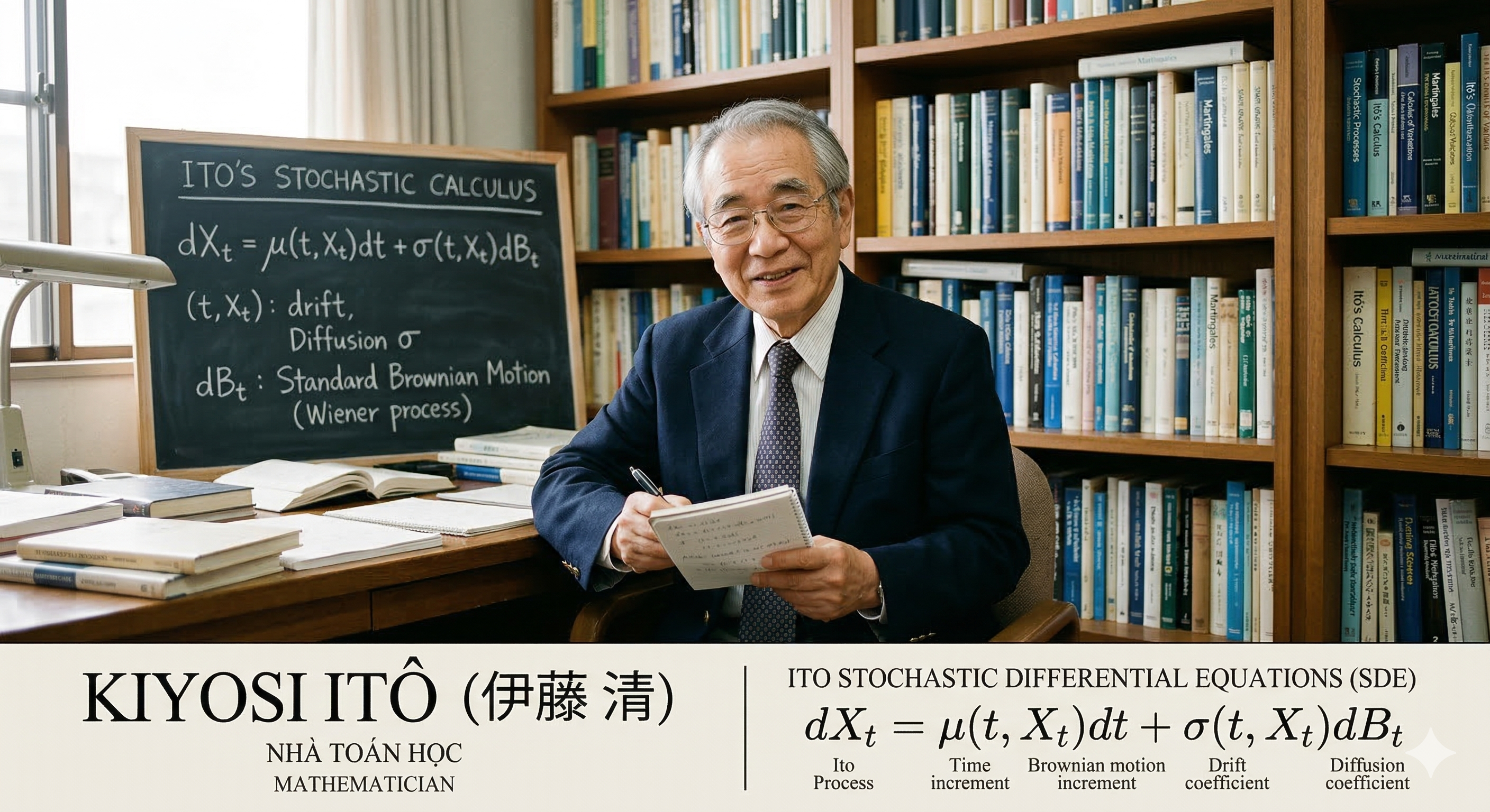
Itô's Stochastic Differential Equation

Itô's Stochastic Differential Equation (SDE) is a mathematical framework for modeling systems that evolve with both deterministic and stochastic components. An SDE can be written in the form: $$d\mathbf{X}_t = \mathbf{f}(\mathbf{X}_t, t) dt + \mathbf{G}(\mathbf{X}_t, t) d\mathbf{W}_t$$ where $\mathbf{X}_t$ is the state of the system at time $t$, $\mathbf{f}$ is the drift term representing deterministic dynamics, $\mathbf{g}$ is the diffusion term representing stochastic dynamics, and $d\mathbf{W}_t$ is a Wiener process (or Brownian motion).

In Diffusion Models, the generative process can be modeled as an SDE where the drift term guides samples toward high-density regions of the data distribution, while the diffusion term adds noise to ensure diversity in generated samples.

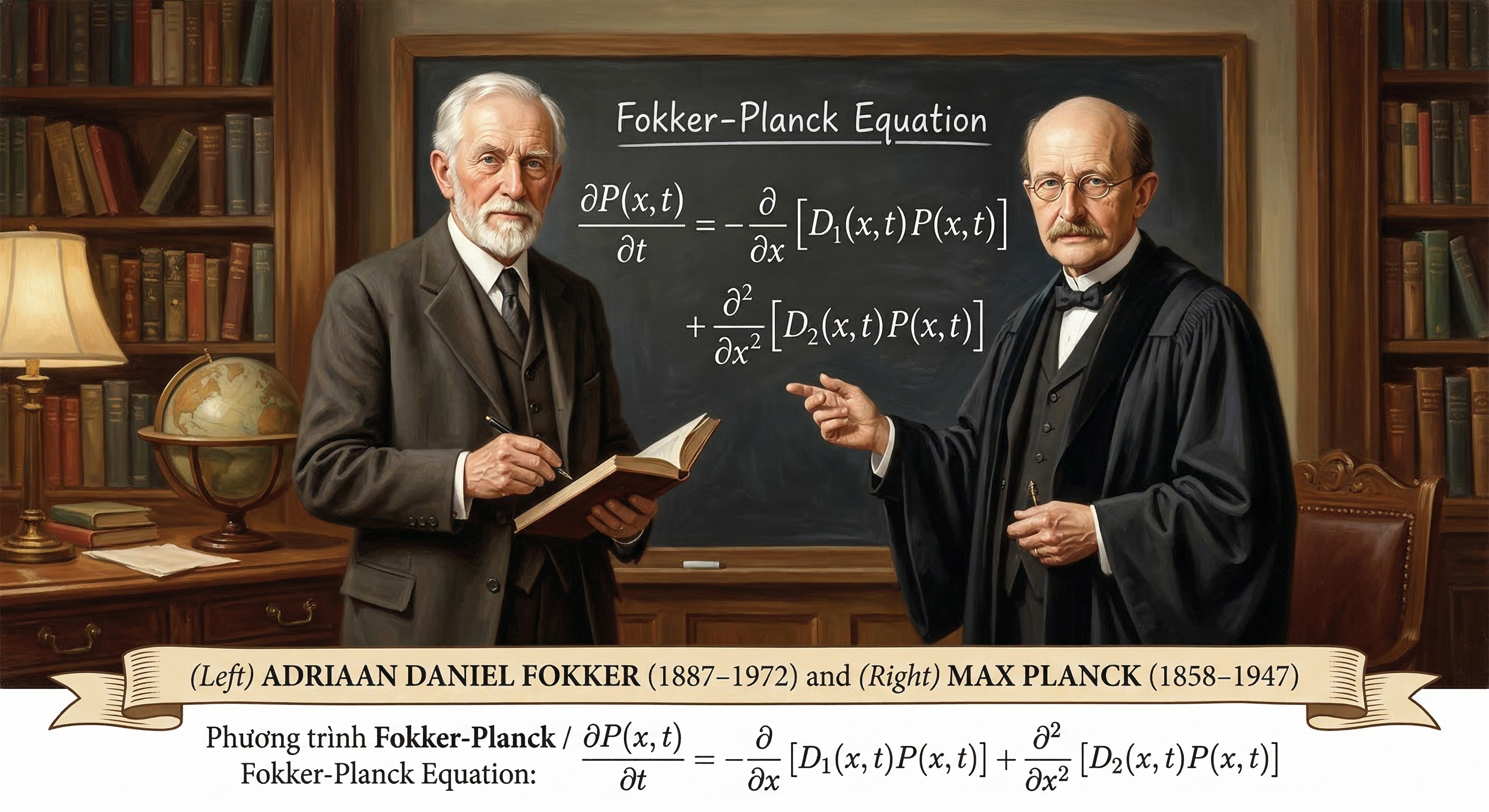
Fokker-Planck Equation

The Fokker-Planck Equation describes the time evolution of the probability density function of a stochastic process governed by an SDE. For an SDE of the form given above, the corresponding Fokker-Planck Equation is: $$\frac{\partial p}{\partial t} = -\nabla \cdot (\mathbf{f} p) + \frac{1}{2} \nabla^2 : (\mathbf{G} \mathbf{G}^T p)$$ where $\nabla^2 :$ denotes the divergence of the diffusion term.

In the context of Diffusion Models, the Fokker-Planck Equation provides a theoretical framework for understanding how the probability density evolves over time under the influence of both deterministic and stochastic forces. It helps us analyze how samples transition from noise to structured data as they are guided by the Score Function and influenced by random perturbations.

Sub-Summary 1

Stokes' Theorem

Stokes' Theorem is a powerful mathematical tool that relates the surface integral of a vector field over a surface $S$ to the line integral of the same vector field around the boundary curve $\partial S$ of that surface. Formally, it can be expressed as: $$\oint_{\partial S} \mathbf{F} \cdot d\mathbf{s} = \iint_S (\nabla \times \mathbf{F}) \cdot d\mathbf{S}$$

Given that the Score Function is defined as the gradient of the log-density, $\mathbf{s} = \nabla \log p$, it inherently constitutes a conservative vector field. A fundamental property of such fields is that their curl is identically zero: $$\nabla \times \mathbf{s} = \nabla \times (\nabla \log p) = 0$$ By invoking Stokes' Theorem, it can be demonstrated that the line integral around any closed loop $C$ vanishes, as it equates to the surface integral of a null curl: $$\oint_C \mathbf{s} \cdot d\mathbf{r} = \iint_S (\nabla \times \mathbf{s}) \cdot d\mathbf{S} = 0$$ This mathematical constraint carries profound implications for model convergence. Should the Score Function exhibit any rotational component ($\text{curl} \neq 0$), data particles propelled by the score would risk becoming trapped in limit cycles, thereby failing to converge toward the true data distribution. Consequently, the 'potential function' nature of the Score Function ensures a pure probability flow, guiding the sampling process directly and efficiently toward the high-density regions of the data manifold.

Sub-Summary 2

Probability mass is conserved. The rate at which probability density $p(\mathbf{x},t)$ changes inside a volume $V$ must equal the net flux $\mathbf{j}$ passing through the boundary $\partial V$. $V$ represents an arbitrary volume in an n-dimensional space (in the context of Diffusion, this space corresponds to your data domain).

To relate the surface flow (Flux) to the internal change (Density), we use Gauss's Theorem: $$\iint_{\partial V} \mathbf{j} \cdot d\mathbf{S} = \iiint_V (\nabla \cdot \mathbf{j}) dV$$ This theorem is the 'key' that allows us to translate a global conservation law into a local differential equation.

Since probability is conserved, the increase inside equals the negative of the outward flux: $$\iiint_V \frac{\partial p}{\partial t} \, dV = - \iint_{\partial V} \mathbf{j} \cdot d\mathbf{S}$$ By applying Gauss's Theorem, we derive the Continuity Equation, ensuring that data points are neither created nor destroyed, only moved: $$\iiint_V \frac{\partial p}{\partial t} \, dV = - \iiint_V (\nabla \cdot \mathbf{j}) \, dV$$ Thus, we arrive at the local form of the Continuity Equation: $$\frac{\partial p_t(\mathbf{x})}{\partial t} = -\nabla \cdot \mathbf{j}(\mathbf{x}, t)$$

The flux $\mathbf{j}$ is generated by the motion of 'data particles' following an Itô Stochastic Differential Equation (SDE): $$d\mathbf{x} = \mathbf{f}(\mathbf{x}, t)dt + \mathbf{G}(t)d\mathbf{w}$$ where $\mathbf{f}$ is the drift term (deterministic part) and $\mathbf{G}(t)d\mathbf{w}$ is the diffusion term (stochastic part).

The total flux $\mathbf{j}$ in this process consists of two parts, deterministic drift and stochastic diffusion: $$\mathbf{j}(\mathbf{x}, t) = \underbrace{\mathbf{f}(\mathbf{x}, t) p_t(\mathbf{x})}_{\text{Drift flux}} - \underbrace{\frac{1}{2} \nabla \cdot [\mathbf{G}\mathbf{G}^T p_t(\mathbf{x})]}_{\text{Diffusion flux}}$$ To introduce the Score Function $s(\mathbf{x}) = \nabla_{\mathbf{x}} \log p_t(\mathbf{x})$, we use the following identity: $$\nabla \cdot (\mathbf{A} p) = p (\nabla \cdot \mathbf{A}) + \mathbf{A} \nabla p \text{ (Mathematical Identity)} $$ Here, $\mathbf{A}$ is the Diffusion Tensor ($\mathbf{A} = \mathbf{G}\mathbf{G}^T$). It represents the structure and correlation of the noise. Assuming the noise $\mathbf{G}$ is constant with respect to space ($\nabla \cdot \mathbf{A} = 0$), and using the log-derivative trick ($\nabla p = p \nabla \log p$), the flux simplifies to: $$\mathbf{j}(\mathbf{x}, t) = \left[ \mathbf{f}(\mathbf{x}, t) - \frac{1}{2} \mathbf{G}\mathbf{G}^T \nabla_{\mathbf{x}} \log p_t(\mathbf{x}) \right] p_t(\mathbf{x})$$ The Final Fokker-Planck Equation. By substituting $\mathbf{j}$ back into the Continuity Equation, we obtain the governing equation for the entire Diffusion process expressed via the Score Function: $$\frac{\partial p_t(\mathbf{x})}{\partial t} = -\nabla \cdot \left( \underbrace{\left[ \mathbf{f}(\mathbf{x}, t) - \frac{1}{2} \mathbf{G}\mathbf{G}^T \nabla_{\mathbf{x}} \log p_t(\mathbf{x}) \right]}_{\text{Velocity Field } \mathbf{v}(\mathbf{x}, t)} p_t(\mathbf{x}) \right)$$

This equation is the mathematical bridge that allows us to replace stochastic uncertainty with deterministic flow. It proves that by simply learning the gradient of the log-density (the Score), a neural network can perfectly simulate the complex evolution of data distributions.

4. Advanced Perspectives

4.1 Flow Matching Framework

If we already have a velocity field defined by the Fokker-Planck equation, why do we still need Flow Matching? The Fokker-Planck equation provides a theoretical framework for understanding how probability densities evolve under the influence of both deterministic and stochastic forces. However, it does not prescribe a specific method for training a neural network to learn this evolution. Flow Matching is a practical framework that allows us to directly train a neural network to match the velocity field defined by the Fokker-Planck equation. It provides a way to optimize the parameters of the neural network so that it can accurately capture the dynamics of the data distribution as it evolves over time.

In Sub-Summary 2, we proof that Fokker-Planck equation can be expressed in terms of the Continuity Equation: $$\frac{\partial p_t(\mathbf{x})}{\partial t} = -\nabla \cdot \left( \mathbf{v}(\mathbf{x}, t) p_t(\mathbf{x}) \right)$$ Where $\mathbf{v}(\mathbf{x}, t) = \mathbf{f}(\mathbf{x}, t) - \frac{1}{2} \mathbf{G}\mathbf{G}^T \nabla_{\mathbf{x}} \log p_t(\mathbf{x})$ is the velocity field that governs the flow of probability density.

This equation asserts that although data particles move randomly (SDE), their density evolves deterministically along a flow. This observation opens up the possibility of replacing the stochastic differential equation with an ordinary differential equation (ODE): $$\frac{d\mathbf{x}}{dt} = \mathbf{v}(\mathbf{x}, t)$$

Neural Ordinary Differential Equations

Probability Paths

Having established that the evolution of data particles can be modeled by an ODE via the Instantaneous Change of Variables theorem, we must define the trajectory they follow. In the context of Flow Matching (Lipman et al., 2024), we focus on Probability Paths. A probability path is a continuous sequence of probability density functions, denoted as $p_t(\mathbf{x})$, for $t \in [0, 1]$.

In generative modeling, we construct a boundary-value problem: the path must transition smoothly from a simple, tractable prior distribution at $t=0$ (e.g., standard Gaussian noise, $p_0 \sim \mathcal{N}(0, \mathbf{I})$) to the complex, unknown empirical data distribution at $t=1$ ($p_1 \approx p_{data}$). The fundamental premise of Flow Matching is to directly engineer a target vector field $\mathbf{v}_t(\mathbf{x})$ that generates this desired probability path $p_t(\mathbf{x})$ through the continuity equation, bypassing the need to approximate the intractable score function $\nabla \log p_t(\mathbf{x})$ mandated by the traditional Fokker-Planck approach.

Flow Matching Framework

Once a target probability path $p_t(\mathbf{x})$ and its corresponding target vector field $\mathbf{v}_t(\mathbf{x})$ are mathematically formulated, the objective is to train a neural network, parameterized by $\theta$, to approximate this field. The model's vector field, $\mathbf{v}_\theta(\mathbf{x}, t)$, is optimized using a straightforward continuous-time regression loss, formally defined as the Flow Matching Objective: $$ \mathcal{L}_{FM}(\theta) = \mathbb{E}_{t \sim \mathcal{U}[0,1], \mathbf{x} \sim p_t(\mathbf{x})} \left[ \| \mathbf{v}_\theta(\mathbf{x}, t) - \mathbf{v}_t(\mathbf{x}) \|^2 \right] $$

However, a critical mathematical bottleneck emerges: computing the marginal target vector field $\mathbf{v}_t(\mathbf{x})$ and sampling directly from the marginal density $p_t(\mathbf{x})$ is computationally intractable. The marginal field requires integrating over the entire dataset simultaneously, which is impossible in high-dimensional spaces with millions of data points. Thus, while $\mathcal{L}_{FM}(\theta)$ is theoretically sound, it cannot be directly minimized in practice.

Conditional Flow Matching

To resolve this intractability, Lipman et al. (2022) introduced a mathematical breakthrough known as Conditional Flow Matching (CFM). Instead of modeling the macroscopic flow of the entire dataset, we condition the probability path on a single data observation $\mathbf{x}_1 \sim q(\mathbf{x}_1)$.

By defining a conditional probability path $p_t(\mathbf{x} | \mathbf{x}_1)$ and its associated conditional vector field $\mathbf{v}_t(\mathbf{x} | \mathbf{x}_1)$, we simplify the problem exponentially. A profound theorem in Flow Matching guarantees that if we average (marginalize) all the conditional vector fields, we perfectly reconstruct the intractable marginal vector field. Consequently, the intractable FM loss can be seamlessly replaced by the tractable Conditional Flow Matching Objective: $$ \mathcal{L}_{CFM}(\theta) = \mathbb{E}_{t, \mathbf{x}_1 \sim q(\mathbf{x}_1), \mathbf{x} \sim p_t(\mathbf{x}|\mathbf{x}_1)} \left[ \| \mathbf{v}_\theta(\mathbf{x}, t) - \mathbf{v}_t(\mathbf{x} | \mathbf{x}_1) \|^2 \right] $$

By replacing the complex, curved stochastic trajectories of standard diffusion (governed by $\mathbf{G}\mathbf{G}^T \nabla \log p_t$) with straight, deterministic Conditional Optimal Transport paths, Flow Matching drastically flattens the optimization landscape. The neural network $\mathbf{v}_\theta$ no longer struggles to predict chaotic noise variations; it simply learns to predict the linear direction $\mathbf{x}_1 - \mathbf{x}_0$, setting the foundation for ultra-fast ODE solvers like DPM-Solver-v3.

4.2 Four Prediction Types Are Equivalent

$\epsilon$-Prediction - Noise Prediction

Instead of requiring the model to directly paint a complete picture, this method trains the neural network to identify and isolate the chaotic noise injected into the data at timestep $t$. $$\hat{\mathbf{x}}_0 = \frac{\mathbf{x}_t - \sigma_t \hat{\boldsymbol{\epsilon}}}{\alpha_t}$$

This approach exhibits outstanding stability in high-noise regimes ($t \to T$). It serves as the gold standard foundational design that underpinned the success of DDPM (Ho et al., 2020) and the Stable Diffusion 1.5 ecosystem. Predicting standard Gaussian noise ensures that the loss function maintains a uniform variance during the initial steps.

As the sampling process approaches the final steps ($t \to 0$, where $\sigma_t \to 0$), even a minuscule approximation error by the neural network in estimating $\hat{\boldsymbol{\epsilon}}$ becomes drastically amplified (due to division by $\alpha_t$ or multiplication by an infinitesimal $\sigma_t$). This numerical instability leads to visual degradation phenomena such as color shifting or artifacts.

$x$-Prediction - Clean Prediction

This approach demands that the neural network possess 'X-ray vision,' enabling it to see through the random, opaque noise layer $\mathbf{x}_t$ and map directly back to the pristine, original image $\mathbf{x}_0$ in a single inference step. $$\hat{\boldsymbol{\epsilon}} = \frac{\mathbf{x}_t - \alpha_t \hat{\mathbf{x}}_0}{\sigma_t}$$

Extremely effective in low-noise regimes ($t \to 0$). It denoises decisively, maintaining the sharpness and global structure of the image. This technique is frequently prioritized in Super-Resolution architectures, Video Generation, or Consistency Models.

It becomes mathematically intractable at maximum noise levels. If forced to interpolate an image from pure white noise, the model tends to predict the mean squared value of the entire training dataset. Consequently, the output becomes blurry, ultimately leading to mode collapse.

Score Prediction

Viewed through the lens of Statistical Physics and directly linked to the Fokker-Planck equation, rather than guessing data or noise, the model estimates the gradient field of the log-probability density function. It acts as a compass pointing in the steepest direction to guide the noise particles back toward the true data manifold. $$\mathbf{s}(\mathbf{x}_t, t) = -\frac{\boldsymbol{\epsilon}}{\sigma_t}$$

Provides the most rigorous and elegant mathematical framework, which is particularly essential for proving convergence theorems in SDEs/ODEs (Song et al., 2021).

Encounters severe issues with Exploding Gradients. As $\sigma_t \to 0$, the value of the Score function approaches infinity. To prevent the neural network from becoming unstable during backpropagation, researchers are compelled to design highly complex Loss Weighting schemes.

$v$-Prediction - Velocity Prediction

$v$-prediction (proposed in Progressive Distillation for Fast Sampling, Salimans & Ho 2022) introduces a quantity $\mathbf{v}$ that acts as a perfect linear interpolation between the clean image space ($\mathbf{x}_0$) and the noise space ($\boldsymbol{\epsilon}$). In the fluid mechanics of diffusion models, it represents the velocity of the data particle as it moves along the trajectory of the Probability Flow ODE (PF-ODE). $$\mathbf{v}_t = \alpha_t \boldsymbol{\epsilon} - \sigma_t \mathbf{x}_0$$

Comprehensively resolves the blind spots of both the $\epsilon$ and $x_0$ coordinate frames. By combining them via trigonometric coefficients $\alpha_t$ and $\sigma_t$, the variance and amplitude of $\mathbf{v}_t$ remain stationary across the entire time spectrum $t \in [0, 1]$. This completely eliminates numerical instability at both extremes of the diffusion process.

This represents a foundational leap, acting as a mandatory prerequisite for ushering in the era of Flow Matching and Rectified Flow (where curved trajectories are straightened). It provides the underlying power for advanced model generations like Stable Diffusion 2.0+ and SD3.

5. Optimal Transport and Schrödinger Bridges

5.1 Schrödinger Bridges

The Schrödinger Bridge is a foundational concept in probability theory, optimal transport, and statistical physics, originally formulated by physicist Erwin Schrödinger in 1931 (Über die Umkehrung der Naturgesetze).

Conceptually, it answers a thought experiment: Imagine you observe a cloud of particles undergoing random motion (like Brownian motion) at time $t=0$ with a specific starting distribution. At a later time $t=T$, you observe them again, but they form a completely different distribution—one that is highly unlikely to have occurred naturally by pure random chance. What is the most probable path those particles took to get from the initial distribution to the final one?

The Schrödinger Bridge finds the most likely sequence of intermediate states, bridging the two distributions with minimal unnatural forcing.

Before applying the bridge, we must establish the 'reference measure' or the prior unconstrained dynamics. In the continuous-time diffusion framework, the baseline motion of data particles is governed by an Itô Stochastic Differential Equation (SDE): $$d\mathbf{x} = \mathbf{f}(\mathbf{x}, t)dt + \mathbf{G}d\mathbf{w}$$ Where $\mathbf{f}(\mathbf{x}, t)$ represents the deterministic drift vector and $\mathbf{G}$ is the diffusion matrix controlling the stochastic noise.

As established by the local form of the Continuity Equation and Gauss's Theorem, probability mass is conserved during this process. The time evolution of the probability density $p_t(\mathbf{x})$ under these reference dynamics is perfectly described by the standard Fokker-Planck Equation: $$\frac{\partial p_t(\mathbf{x})}{\partial t} = -\nabla \cdot \left( \left[ \mathbf{f}(\mathbf{x}, t) - \frac{1}{2} \mathbf{G}\mathbf{G}^T \nabla_{\mathbf{x}} \log p_t(\mathbf{x}) \right] p_t(\mathbf{x}) \right)$$ In this unconstrained state, the velocity field guiding the probability flow is naturally $\mathbf{v}(\mathbf{x}, t) = \mathbf{f}(\mathbf{x}, t) - \frac{1}{2} \mathbf{G}\mathbf{G}^T \nabla_{\mathbf{x}} \log p_t(\mathbf{x})$.

The Schrödinger Bridge Problem imposes two strict boundary conditions: an initial distribution $p_0(\mathbf{x})$ and a specific, complex target distribution $p_T(\mathbf{x})$. The goal is to find a new stochastic process that exactly bridges these two distributions in finite time $T$, while minimizing the Kullback-Leibler (KL) divergence with respect to the reference SDE defined above.

To force the particles to reach $p_T$ instead of diffusing endlessly into noise, we must apply an external 'control force' to the drift. According to stochastic control theory and the Hopf-Cole transformation, the optimal controlled SDE that solves the Schrödinger Bridge takes the following form: $$d\mathbf{x} = \left[ \mathbf{f}(\mathbf{x}, t) + \mathbf{G}\mathbf{G}^T \nabla_{\mathbf{x}} \log \Psi(\mathbf{x}, t) \right] dt + \mathbf{G}d\mathbf{w}$$ Here, $\Psi(\mathbf{x}, t)$ is a scalar function known as the forward Schrödinger potential. The term $\mathbf{G}\mathbf{G}^T \nabla_{\mathbf{x}} \log \Psi(\mathbf{x}, t)$ represents the precise, minimal mathematical guidance required to steer the probability flow toward the destination distribution.

The Schrödinger-Fokker-Planck Equation

When we inject this optimal, controlled drift back into the continuity framework, the fundamental velocity field driving the density changes. We substitute the new drift $\mathbf{f}_{SB} = \mathbf{f} + \mathbf{G}\mathbf{G}^T \nabla \log \Psi$ into the flux equation. The updated velocity field for the Schrödinger Bridge becomes: $$\mathbf{v}_{SB}(\mathbf{x}, t) = \mathbf{f}(\mathbf{x}, t) + \mathbf{G}\mathbf{G}^T \nabla_{\mathbf{x}} \log \Psi(\mathbf{x}, t) - \frac{1}{2} \mathbf{G}\mathbf{G}^T \nabla_{\mathbf{x}} \log p_t(\mathbf{x})$$ Consequently, the modified Fokker-Planck Equation governing the precise evolution of the bridged density is: $$\frac{\partial p_t(\mathbf{x})}{\partial t} = -\nabla \cdot \left( \left[ \mathbf{f}(\mathbf{x}, t) + \mathbf{G}\mathbf{G}^T \nabla_{\mathbf{x}} \log \Psi(\mathbf{x}, t) - \frac{1}{2} \mathbf{G}\mathbf{G}^T \nabla_{\mathbf{x}} \log p_t(\mathbf{x}) \right] p_t(\mathbf{x}) \right)$$

System of Coupled Potentials

Unlike standard diffusion models that only require learning a single score function $\nabla_{\mathbf{x}} \log p_t(\mathbf{x})$ pointing toward the data manifold, solving the SB-modified Fokker-Planck equation requires modeling the interaction between the start and end points simultaneously. The probability density at any intermediate time $t$ in a Schrödinger Bridge is mathematically factored into the product of two distinct potentials: $$p_t(\mathbf{x}) = \Psi(\mathbf{x}, t) \hat{\Psi}(\mathbf{x}, t)$$

• $\Psi(\mathbf{x}, t)$ is the forward potential (ensuring the system respects the prior dynamic structure).
• $\hat{\Psi}(\mathbf{x}, t)$ is the backward potential (acting as the gravitational pull of the target distribution $p_T$).

The Substitution

If we substitute these new SB components into the velocity field equation, we get: $$\mathbf{v}_{SB}(\mathbf{x}, t) = \underbrace{\mathbf{f}(\mathbf{x}, t) + \mathbf{G}\mathbf{G}^T \nabla_{\mathbf{x}} \log \Psi(\mathbf{x}, t)}_{\text{New Controlled Drift}} - \frac{1}{2} \mathbf{G}\mathbf{G}^T \nabla_{\mathbf{x}} \log \big( \Psi(\mathbf{x}, t) \hat{\Psi}(\mathbf{x}, t) \big)$$ Because the logarithm of a product is the sum of the logarithms, we can expand the gradient of the log-density: $$\nabla_{\mathbf{x}} \log p_t = \nabla_{\mathbf{x}} \log \Psi + \nabla_{\mathbf{x}} \log \hat{\Psi}$$ Substitute this expansion back into the velocity equation: $$\mathbf{v}_{SB}(\mathbf{x}, t) = \mathbf{f} + \mathbf{G}\mathbf{G}^T \nabla_{\mathbf{x}} \log \Psi - \frac{1}{2} \mathbf{G}\mathbf{G}^T \nabla_{\mathbf{x}} \log \Psi - \frac{1}{2} \mathbf{G}\mathbf{G}^T \nabla_{\mathbf{x}} \log \hat{\Psi}$$ Combine the $\nabla_{\mathbf{x}} \log \Psi$ terms: $$\mathbf{v}_{SB}(\mathbf{x}, t) = \mathbf{f} + \frac{1}{2} \mathbf{G}\mathbf{G}^T \nabla_{\mathbf{x}} \log \Psi - \frac{1}{2} \mathbf{G}\mathbf{G}^T \nabla_{\mathbf{x}} \log \hat{\Psi}$$Factor out the $\frac{1}{2} \mathbf{G}\mathbf{G}^T$: $$\mathbf{v}_{SB}(\mathbf{x}, t) = \mathbf{f}(\mathbf{x}, t) + \frac{1}{2} \mathbf{G}\mathbf{G}^T \Big( \nabla_{\mathbf{x}} \log \Psi(\mathbf{x}, t) - \nabla_{\mathbf{x}} \log \hat{\Psi}(\mathbf{x}, t) \Big)$$ Using the logarithm quotient rule, we arrive at the final, simplified velocity field.

Practical Implementation via IPF

Analytically solving this modified Fokker-Planck equation for high-dimensional data (like images) is mathematically intractable. In modern machine learning, this is resolved using the Diffusion Schrödinger Bridge (DSB) framework.

Instead of solving the PDEs directly, DSB approximates the solution using an algorithm called Iterative Proportional Fitting (IPF). IPF trains two separate neural networks—one to estimate the forward drift and one to estimate the backward drift—and alternates simulating forward SDE trajectories and backward SDE trajectories. Through successive half-iterations (simulating forward to update the backward network, then backward to update the forward network), the modeled velocity field progressively aligns with the theoretical $\mathbf{v}_{SB}(\mathbf{x}, t)$, granting the ability to map between domains with exceptional efficiency.

5.2 Optimal Transport as a Special Case of Schrödinger Bridges

The Dynamic Formulation of Optimal Transport

To see the connection, we must look at Optimal Transport not through static maps, but through its dynamic formulation, famously known as the Benamou-Brenier formula (Martin Huesmann and Bastian Muller).

magine moving a pile of sand (distribution $p_0$) to a hole (distribution $p_T$) over a time interval $t \in [0,T]$. Standard OT seeks the absolute 'cheapest' flow—minimizing the kinetic energy of the transport without any random scattering of the sand.

Formula for OT (Benamou-Brenier): $$W_2^2(p_0, p_T) = \inf_{\rho, \mathbf{v}} \int_0^T \int_{\mathbb{R}^d} \frac{1}{2} \|\mathbf{v}(\mathbf{x}, t)\|^2 \rho(\mathbf{x}, t) d\mathbf{x} dt$$ ubject to the Continuity Equation (deterministic flow):$$\frac{\partial \rho}{\partial t} + \nabla \cdot (\rho \mathbf{v}) = 0$$ With boundary conditions: $\rho(\mathbf{x}, 0) = p_0(\mathbf{x})$ and $\rho(\mathbf{x}, T) = p_T(\mathbf{x})$. n this deterministic model, the equivalent SDE describing particle motion has no noise: $$d\mathbf{x} = \mathbf{v}(\mathbf{x}, t)dt$$

The Schrödinger Bridge (Entropy-Regularized OT)

The Schrödinger Bridge tackles the exact same goal (moving from $p_0$ to $p_T$), but it assumes the particles are naturally undergoing Brownian motion (diffusion). Therefore, the transport plan must balance minimizing the transport effort (kinetic energy) against the natural dispersion (entropy).

Let $\epsilon > 0$ represent the variance of the diffusion process (the 'temperature' or noise level).

Formula for Schrödinger Bridge: $$SB_\epsilon(p_0, p_T) = \inf_{\rho, \mathbf{v}} \int_0^T \int_{\mathbb{R}^d} \frac{1}{2} \|\mathbf{v}(\mathbf{x}, t)\|^2 \rho(\mathbf{x}, t) d\mathbf{x} dt$$ Subject to the Fokker-Planck Equation (stochastic flow): $$\frac{\partial \rho}{\partial t} + \nabla \cdot (\rho \mathbf{v}) = \epsilon \Delta \rho$$ (Note: $\Delta \rho$ is the Laplacian, which is equivalent to $\nabla \cdot \nabla \rho$, representing the diffusion term).

With the same boundary conditions: $\rho(\mathbf{x}, 0) = p_0(\mathbf{x})$ and $\rho(\mathbf{x}, T) = p_T(\mathbf{x})$. In this stochastic model, the equivalent SDE describing particle motion includes a Wiener process (noise) scaled by $\epsilon$: $$d\mathbf{x} = \mathbf{v}(\mathbf{x}, t)dt + \sqrt{2\epsilon} d\mathbf{w}_t$$

The Limit Theorem

The structural equivalence between the two formulas is exact, differing only in the constraint governing the density evolution (Continuity vs. Fokker-Planck). The formal relationship is defined by taking the limit of the Schrödinger Bridge as the noise parameter $\epsilon$ goes to $0$: $$\lim_{\epsilon \to 0} SB_\epsilon(p_0, p_T) = W_2^2(p_0, p_T)$$

6. Sampling and Control

Having established the rigorous mathematical foundations of probability flows and vector fields in previous sections, we now shift our focus to operational steering mechanisms. If Sections 2 through 5 delineate how the generative 'flow' operates, Section 6 elucidates how we can precisely navigate this trajectory toward desired outcomes—be they semantic adherence, aesthetic quality, or structural constraints.

6.1 Classifier-Free Guidance

Building upon the concept of the Score Function ($\nabla_{\mathbf{x}} \log p(\mathbf{x})$) introduced in Section 2.3, we introduce the paradigm of the Conditional Score. Historically, Classifier Guidance necessitated an auxiliary, pre-trained classification model to direct the generation process. Classifier-Free Guidance (CFG) elegantly circumvents this dependency by interpolating between a conditional score (e.g., guided by a text prompt, $c$) and an unconditional score ($\emptyset$).

The mathematical formulation is expressed as: $$\mathbf{\hat{s}}_\theta(\mathbf{x}_t, c) = \mathbf{s}_\theta(\mathbf{x}_t, \emptyset) + w \cdot (\mathbf{s}_\theta(\mathbf{x}_t, c) - \mathbf{s}_\theta(\mathbf{x}_t, \emptyset))$$ Here, the guidance scale $w$ acts as a scalar amplifier for the vector pointing from the unconditional noise distribution toward the conditioned data manifold. While a higher $w$ significantly enhances prompt fidelity—ensuring the output closely aligns with user constraints—it inherently incurs a trade-off by diminishing the overall diversity of the generated samples.

6.2 Direct Preference Optimization

While Schrödinger Bridges (Section 5) optimize the trajectory between two distributions, Direct Preference Optimization (Wallace et al., 2023) fine-tunes these pathways to satisfy human aesthetic or semantic preferences. DPO shifts the objective from maximum likelihood estimation (simply reconstructing data) to modeling human choices based on the Bradley-Terry preference framework.

The fundamental bottleneck in applying DPO to Diffusion Models lies in the intractability of directly computing the log-likelihood $\log p_\theta(\mathbf{x})$. To resolve this, we leverage the equivalence of parametrizations (Section 4.2), approximating the log-likelihood via the Denoising Score Matching objective (the Evidence Lower Bound, or ELBO): $$\log p_\theta(\mathbf{x} \mid c) \approx -\mathbb{E}_{t, \boldsymbol{\epsilon}} \left[ w(t) \| \boldsymbol{\epsilon} - \boldsymbol{\epsilon}_\theta(\mathbf{x}_t, t, c) \|_2^2 \right] + C$$ By substituting this approximation into the DPO formulation, we elegantly translate human preference into a 'push-pull' mechanism operating directly on the vector field:

• Attraction (Pull): The model is optimized to minimize the noise prediction error for the preferred sample ($\mathbf{x}_w$), actively modifying the velocity field to increase the probability of generating this specific trajectory.
• Repulsion (Push): Conversely, it penalizes the trajectory of the rejected sample ($\mathbf{x}_l$), pushing the vector field away from undesirable outcomes.

6.3 Training-Free Guidance

Once a highly optimized velocity field is established, a compelling question arises: how can we intervene during the sampling phase without incurring the prohibitive computational costs of retraining? Training-Free Guidance provides sophisticated mathematical interventions to manipulate the generation process post-hoc.

• Self-Guidance: This technique exploits the internal representations of the pre-trained architecture—such as cross-attention maps within a UNet or Transformer—to spatially constrain objects or enforce structural coherence during the denoising steps.
• Energy-Based Guidance: By introducing the gradient of an external energy function $E(\mathbf{x})$ directly into the sampling equation, we can mathematically perturb the trajectory:$$\mathbf{x}_{t-1} = \text{SolverUpdate}(\mathbf{x}_t) - \eta \nabla_{\mathbf{x}} E(\mathbf{x}_t)$$This acts as an auxiliary force field, steering the data particles toward states of lower 'energy' (representing desired attributes like specific color palettes, physical plausibility, or semantic safety).
• Architectural Reweighting (e.g., FreeU): Advanced methods strategically reweight the low-frequency (semantic) and high-frequency (detail) components within the model's skip connections during inference. This substantially enhances visual fidelity and structural integrity without requiring any additional training epochs.

7. Sophisticated Solvers

The journey from continuous-time diffusion theory to practical, ultra-fast sampling algorithms represents one of the most elegant mathematical flows in generative AI. By understanding how probability density evolves, we can derive exact deterministic trajectories and strategically approximate them for rapid generation.

As established, the forward diffusion process can be described by an Itô Stochastic Differential Equation (SDE): $$ d\mathbf{x} = \mathbf{f}(\mathbf{x}, t) dt + g(t) d\mathbf{w} $$ The time evolution of the probability density $p_t(\mathbf{x})$ for this SDE is governed by the Fokker-Planck Equation: $$ \frac{\partial p_t(\mathbf{x})}{\partial t} = -\nabla \cdot (\mathbf{f}(\mathbf{x}, t) p_t(\mathbf{x})) + \frac{1}{2} g(t)^2 \nabla^2 p_t(\mathbf{x})$$

A remarkable property of diffusion models is that we can construct a deterministic Ordinary Differential Equation (ODE) whose marginal distributions exactly match those of the SDE. By matching the terms of the Fokker-Planck equation, we arrive at the corresponding Probability Flow ODE: $$ d\mathbf{x} = \left[ \mathbf{f}(\mathbf{x}, t) - \frac{1}{2} g(t)^2 \nabla_{\mathbf{x}} \log p_t(\mathbf{x}) \right] dt $$ Notice the presence of the score function, $\nabla_{\mathbf{x}} \log p_t(\mathbf{x})$. In standard Diffusion Probabilistic Models (DPMs), the drift is linear, defined as $\mathbf{f}(\mathbf{x}, t) = f(t)\mathbf{x}$. By substituting the score function with our learned noise predictor using the relation $\nabla_{\mathbf{x}} \log p_t(\mathbf{x}) = -\frac{\epsilon_\theta(\mathbf{x}_t, t)}{\sigma_t}$, we obtain the practical diffusion ODE: $$ \frac{d\mathbf{x}_t}{dt} = f(t)\mathbf{x}_t + \frac{g^2(t)}{2\sigma_t} \epsilon_\theta(\mathbf{x}_t, t) $$

Solving this ODE numerically poses a challenge because the neural network $\epsilon_\theta$ is highly non-linear, traditionally requiring hundreds of evaluations. However, the ODE possesses a distinct semi-linear structure.

By changing the time variable $t$ to the log-SNR (Signal-to-Noise Ratio) domain, defined as $\lambda_t = \log(\alpha_t / \sigma_t)$, the ODE simplifies. Applying the variation of constants formula—a core principle of exponential integrators—allows us to compute the linear part of the ODE exactly. The exact solution becomes: $$ \mathbf{x}_t = \frac{\alpha_t}{\alpha_s} \mathbf{x}_s - \alpha_t \int_{\lambda_s}^{\lambda_t} e^{-\lambda} \hat{\epsilon}_\theta(\mathbf{x}_\lambda, \lambda) d\lambda $$ This profound simplification reduces the sampling problem from integrating a complex differential equation to merely approximating the integral of the non-linear neural network component.

7.1 DPM-Solver/DPM-Solver++/DPM-Solver-v3

DPM-Solver: Fast Sampling via Taylor Expansion

Instead of applying standard, generic numerical solvers to the integral, the DPM-Solver family (Lu et al., 2022) leverages the analytical properties of the neural network. It approximates the integral by taking a Taylor expansion of the noise predictor $\epsilon_\theta$ with respect to the log-SNR $\lambda$.

Because $\lambda$ naturally tracks the schedule of the diffusion process, treating the neural network output as a polynomial in $\lambda$ vastly reduces the discretization error. This mathematical insight allows DPMs to jump across time steps, generating high-quality samples in as few as 10 to 20 function evaluations (NFE).

DPM-Solver++: Stabilizing Guided Sampling

While DPM-Solver achieves extreme speedups for unconditional generation, it suffers from instability when paired with large classifier-free guidance scales. High guidance scales amplify both the output and the derivatives of the noise prediction model, drastically narrowing the solver's convergence radius.

To solve this, DPM-Solver++ (Lu et al., 2022) reformulates the exact ODE solution to integrate over the data prediction model $\mathbf{x}_\theta$ rather than the noise predictor $\epsilon_\theta$. The data predictor is defined as $\mathbf{x}_\theta(\mathbf{x}_t, t) = (\mathbf{x}_t - \sigma_t \epsilon_\theta(\mathbf{x}_t, t)) / \alpha_t$. The exact solution transforms into: $$ \mathbf{x}_t = \frac{\sigma_t}{\sigma_s} \mathbf{x}_s + \sigma_t \int_{\lambda_s}^{\lambda_t} e^{\lambda} \hat{\mathbf{x}}_\theta(\mathbf{x}_\lambda, \lambda) d\lambda $$ By applying the Taylor expansion to $\mathbf{x}_\theta$ instead, DPM-Solver++ mitigates the instability. Furthermore, it seamlessly accommodates dynamic thresholding methods, ensuring that the converged solutions remain perfectly within the valid data boundaries to prevent 'train-test mismatch' saturation.

DPM-Solver-v3: Empirical Model Statistics (EMS)

The mathematical evolution culminates with DPM-Solver-v3 (Zheng et al., 2023). This iteration challenges the assumption that we must rigidly choose between pure noise prediction or pure data prediction. Instead, it introduces a generalized ODE formulation containing three undetermined coefficients ($l_\lambda, s_\lambda, b_\lambda$): $$ \mathbf{x}_{\lambda_t} = \alpha_{\lambda_t} e^{-\int_{\lambda_s}^{\lambda_t} l_\lambda d\lambda} \left( \frac{\mathbf{x}_{\lambda_s}}{\alpha_{\lambda_s}} - \int_{\lambda_s}^{\lambda_t} e^{\int_{\lambda_s}^{\lambda} (l_\tau + s_\tau) d\tau} \left( \mathbf{g}_\theta(\mathbf{x}_\lambda, \lambda) + \int_{\lambda_s}^{\lambda} e^{-\int_{\lambda_s}^{\tau} s_r dr} b_\tau d\tau \right) d\lambda \right) $$

By analyzing the first-order discretization error, DPM-Solver-v3 isolates the optimal set of these coefficients that strictly minimize the approximation error. Because these optimal coefficients depend directly on the pre-trained neural network's Jacobian, they are pre-computed on a small batch of data as Empirical Model Statistics (EMS).

This dynamic parameterization smoothly transitions the solver's focus from data prediction to noise prediction as sampling proceeds, squeezing maximum efficiency out of the ODE and pushing high-fidelity generation limits down to an unprecedented 5 to 10 steps.

8. Consistency Models

8.1 Consistency Functions

While numerical ODE solvers are inherently bottlenecked by truncation errors due to their step-by-step nature, Consistency Models (Song et al., 2023) introduce a fundamental paradigm shift. Instead of approximating a vector field ($\mathbf{v}_\theta \approx \frac{d\mathbf{x}}{dt}$), CMs learn a global mapping function $f_\theta(\mathbf{x}_t, t)$ that teleports any point on the Probability Flow ODE (PF-ODE) trajectory directly to the origin (clean data $\mathbf{x}_0$).

A robust consistency function must strictly satisfy two mathematical constraints:

1. Self-Consistency: $f_\theta(\mathbf{x}_t, t) = f_\theta(\mathbf{x}_{t'}, t') = \mathbf{x}_0$ for all $t, t' \in [0, T]$.
2. Boundary Condition: $f_\theta(\mathbf{x}_0, 0) = \mathbf{x}_0$.

8.2 Training Mechanism

The core training objective compels the neural network to maintain self-consistency across adjacent points along the ODE trajectory. By utilizing an ODE solver to generate adjacent pairs $(\mathbf{x}_{t_{n+1}}, \hat{\mathbf{x}}_{t_n})$, the consistency loss minimizes the discrepancy between their respective mappings: $$\mathcal{L}(\theta, \theta^-) = \mathbb{E} \left[ d \Big( f_\theta(\mathbf{x}_{t_{n+1}}, t_{n+1}) \; , \; f_{\theta^-}(\hat{\mathbf{x}}_{t_n}, t_n) \Big) \right]$$ Crucially, $\theta^-$ denotes the Exponential Moving Average (EMA) of the model weights. This acts as a target network to prevent divergence and stabilize the training dynamics.

Advanced Extension (CTM): To circumvent the loss of high-frequency details caused by jumping directly to $t=0$, Consistency Trajectory Models (CTM) generalize this approach. They define a mapping $G_\theta(\mathbf{x}_t, t, s)$ that allows traversing from $t$ to any arbitrary time $s$ ($0 \le s < t$), offering an optimal trade-off between real-time inference (1 step) and premium visual fidelity (multi-step).

9. Conclusion

In this blog post, we have explored the mathematical foundations of Diffusion Models, starting from the concept of vector fields and score functions, to the role of divergence and the continuity equation in modeling probability flow. We also delved into advanced perspectives such as flow matching frameworks, optimal transport, Schrödinger bridges, sampling techniques, and sophisticated solvers. By understanding these underlying principles, we can better appreciate the power and flexibility of Diffusion Models in generative modeling tasks.